¹Physics and Physical Oceanography Department, Memorial University Newfoundland, St. John’s, NL, Canada ²Process Engineering Department, Memorial University Newfoundland, St. John’s, NL, Canada

*Corresponding author: John Shirokoff, Process Engineering Department, Memorial University Newfoundland, St. John’s, NL, Canada A1C5S7.

Received: November 10, 2019 Published: November 26, 2019

ABSTRACT

Computer controlled X-ray diffraction (XRD) spectra of asphalt binders were studied with respect to X-ray background type, profile fit and dimensional analysis. Four different background (linear, parabolic, 3^rd and 4^th order polynomial) types were used in order to assess profile fit (precision, residual error) the precision of fit and residual error of fit. Pearson VII, pseudo-Voigt, generalized Fermi mathematical functions were employed in this analysis. When varying the Pearson VII exponent (1.6, 2.0) and pseudo-Voigt Lorentzian at constant value (1.0) the results show an effect on the X-ray peak position and calculated average size of crystallite parameters. Interlayer distance between aromatic sheets (d_M) was determined to be between 4.3 to 4.8 angstroms and the distance between the saturated portions (d_γ) at 5.7 to 6.9 angstroms. For all cases the lowest residual error of fit was the 4^th order polynomial X-ray background type.

Keywords: Asphalt binder; X-ray diffraction; Spectral line shapes; Fitting; Plotting; Modeling

INTRODUCTION

Asphaltene found in asphalt binders is a brown to black colored chemical component of hydrocarbons. The most common forms of asphaltene are petroleum refined as a residue of distillation followed by natural deposits e.g. Trinidad Lake [1].

Asphalt binder and asphalt structure and chemistry are important aspects of crude oils. Separating crude oil in the laboratory results in SARA: saturates, aromatics, resins and asphaltene. The asphaltene consists of aliphatic or paraffin molecular chains, high hydrogen to carbon saturated rings, aromatic unsaturated rings including metals and heteroatoms.

Asphaltene in the form of asphalt binder and asphalt has multiple used not only as a fuel supply but also as asphalt cement for roads and highways, and as roofing materials.

The characterization of asphalt binder has involved various analytical techniques using X-rays, neutrons, electrons, and magnetic radiation. X-ray diffraction (XRD) is popular for studying multiple chemical phases (e.g. asphaltene, wax, metal etc.) present in asphalt binders. This paper is aimed at analyzing the X-ray spectral line shapes of asphalt binders by measuring aromaticity and crystallite parameters of asphalt binders chemistry and structure.

MATERIALS AND METHODS

In this research study the samples of asphalt binder samples were obtained from Alberta, Canada crude oil [2]. Samples were coated on glass slides and heated for 10 minutes at 150°C in an oven then cooled to room temperature (25°C).

XRD patterns were obtained using a Rigaku Dmax 2200V-PC and Jade software (version 6.1) [2]. The XRD operated at 40 KV and 40 mA, scan rate of 0.001° 2θ per second and 5 seconds/step detector count time. The patterns were peak searched 5° to 110° (K-alpha-2 removed). Profile fitting in Jade (Pearson VII, pseudo-Voigt; four background types; 5° to 35° 2θ and 60° to 110° 2θ). The XRD data was modeled using Generalized Fermi function (GFF) in Mathematica^TM and compared to the XRD profile fits (Pearson VII, pseudo-Voigt).

Aromaticity:

f_a = C_graphene/(C_graphene + C_γ) = Area_graphene/(Area_graphene+Area_γ)---(1)

Crystallite Parameters:

Interlayer distance between the aromatic sheets: d_M = λ/(2sinθ)---(2)

Interchain layer distance: d_γ = 5λ/(8sinθ)---(3)

Equations (1) to (3) are treated differently due to the background in figures 1 to 3 from mathematical function.

Figure 1. Top to bottom the XRD background types: linear, parabolic, 3^rd order polynomial, and 4^th order polynomial [3, 4].

RESULTS AND DISCUSSION

X-ray Diffraction (XRD) Patterns

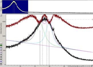
The XRD patterns obtained from the samples consists of four peaks: first peak gamma (γ), second peak (002) graphene, third peak (100), and fourth peak (110) as seen in figures 2 and 3. The peaks in the XRD pattern (10) and (11) correspond to the cubic unit cell planes (100) and (110) indicated in the low half of figure 2. Figure 3 also shows how the effect of X-ray background on the profile fitting in a given sample is performed.

Table 1: The effect of X-ray background on the profile fitting in samples labeled as numbers (No.) 1 to 3.

Sample No.	Math Function	Background	Residual Error of Fit %
1	Pseudo-Voigt	Linear/Parabolic/ 3rd and /4th Order Polynomial	8.3/8.1/8.3/5.1
2	Pseudo-Voigt	Linear/Parabolic/ 3rd and /4th Order Polynomial	7.3/6.2/6.6/5.0
3	Pseudo-Voigt	Linear/Parabolic/ 3rd and /4th Order Polynomial	9.2/10.3/8.9/5.3
1	Pearson VII	Linear/Parabolic/ 3rd and /4th Order Polynomial	8.7/8.1/7.4/7.0
2	Pearson VII	Linear/Parabolic/ 3rd and /4th Order Polynomial	7.5/7.0/6.7/5.0
3	Pearson VII	Linear/Parabolic/ 3rd and /4th Order Polynomial	6.7/9.8/7.3/6.7

Influence of Peak Shape Functions

The XRD peak profile fitting using mathematical function (Pearson VII, pseudo-Voigt) create different peak shapes. Pseudo-Voigt can be pure Gaussian, pure Lorentzian, or a combination of Gaussian and Lorentzian (figure 4) [5, 6].

Pearson VII has an intensity distribution similar to pseudo-Voigt, when β = 1 Pearson VII is Lorentzian, β = 10 Pearson VII peak shape extends outside the range for Gaussian or Lorentzian. Most often Pearson VII represents an exponential mix (Gaussian, Lorentzian). The peak shapes are clearly illustrated in figure 4 for Gauss and Lorentz [6].

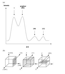
Figure 2.   XRD pattern and peaks (a), and planes they represent (b) [2].

           

Figure 3.   XRD pattern, Pearson VII profile fit (left); GFF-mathematica^TM profile fit (right). Both profiles used a linear type of X-ray background.

Functions (Gauss, Lorentz, pseudo-Voigt, Pearson VII and Generalized Fermi):

Gauss: y(x) = G(x) = (C_G ^1/2)/(√πH) exp (-C_G x²)---(4)

Lorentz: y(x) = L(x) = (C_L ^1/2)/(πH') (1+C_L x²)^-1---(5)

Pseudo-Voigt: y(x) = η (C_G ^1/2)/(√πH) exp (-C_G x²) + (1-η) (C_L ^1/2)/(πH') (1+C_L x²)^-1---(6)

Pearson VII: y(x) = PVII(x) = Γ(β)/(Γ(β)-1/2) (C_P  ^1/2)/(√πH) (1+C_P x²)^-β---(7)

Generalized Fermi: y(x) = A/[exp(-a(x-c))+ exp(b(x-c))]---(8)

Full widths at half maximum (FWHM) are H and H', and x = (2θ_i-2θ_k)/H_k, corresponding to 2θ_i at the origin i^th point and 2θ_i at the k^th point respectively [6].

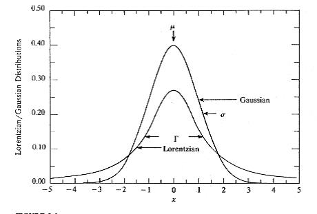
Figure 4.   Lorentzian and Gaussian distributions [5].

The peak shape functions are shown graphically in figure 4. They describe a Gauss function that appears taller at the top relative to the Lorentz function that appears shorter in height. The Lorentz consists of a wider bottom relative to the Gauss. Both Gauss and Lorentz functions are symmetric G(x) = G(-x) and L(x) = L(-x) [7].

The X-ray background intensity is an important feature in line profile analysis since the line profile portion at the bottom of the curve (at high 2θ angles in this data) has some overlap of profiles leading to apparent background intensity [7]. This type of condition can lead to increased error in structural parameters obtained from line profile analysis. Usually a linear background under the profile is assumed from the height and slope as calculated by a straight line from the extremities of the profile over a given measurement range. For relative determinations this is usually not a serious problem.

Table 2: Aromaticity (f_a) and crystallite parameters (d_M the interlayer distance between the aromatic sheets and d_γ the interchain layer distance) for Pearson VII (P) varying exponent (1.6, 2.0), pseudo-Voigt (V) Lorentzian (1.0) constant and Generalized Fermi (GF) Function in samples (S) numbers (No) 1 to 3 using an X-ray background of 4^th order polynomial.

S.	Variable			fa						dM		(Ǻ)				dγ		(Ǻ)
No	Exp. Lor.	P	V		GF		P		V		GF		P		V		GF
1	E1.6 L1.0	0.5	0.4		0.9		4.5		4.5		4.5		5.9		5.9		5.7
2	E1.6 L1.0	0.4	0.4		0.8		4.5		4.5		4.8		6.4		6.4		6.0
3	E1.6 L1.0	0.6	0.6		0.9		4.5		4.5		4.5		6.4		6.9		5.7
1	E2.0 L1.0	0.6	0.4		0.8		4.5		4.3		4.5		5.9		5.7		5.9
2	E2.0 L1.0	0.4	0.4		0.8		4.5		4.5		4.6		6.5		6.2		6.1
3	E2.0 L1.0	0.4	0.5		0.9		4.8		4.5		4.5		6.8		6.6		6.1

Comparing profiles from Jade software to modeling in MathematicaTM the types of X-ray background intensity can affect the calculated results for aromaticity and crystallite parameters as observed from the values of residual error of fit % in table 1. The low to high rank for residual error of fit % was 4^th order polynomial < 3^rd order polynomial < parabolic (4 of 6 data points) < linear background using the materials and methods found in this research paper.

The XRD data modeled by GFF generated a smooth shape (Figure 3). The analysis of aromaticity, dM and dγ parameters (Table 2) showed a strong correlation in spite of asymmetry in the XRD data and four types of background intensity employed (Table 1).

CONCLUSION

XRD patterns obtained and profile fitting using Jade software with Pearson VII and pseudo-Voigt mathematical functions were compared to data modeled by a generalized Fermi function in Mathematica^TM. The crystallite parameter results showed a strong correlation for variations in Pearson VII exponent and pseudo-Voigt Lorentzian when compared to aromaticity. Results are discussed in terms of the measurement and calculation of X-ray background types, intensity, peak shape, profile fit, asymmetry in XRD data and residual error of fit %.

Acknowledgements

The authors would like to thank the Canadian Foundation for Innovation (CFI) and Memorial University of Newfoundland for providing an X-ray laboratory and computing software and facilities to perform the research in this paper. Two of the authors (Ja. A. and Ji. A.) are recipients of graduate student scholarships from the Government of Saudi Arabia.

Conflict of Interest: The authors declare no conflict of interest.

REFERENCES

1. K. Akbarzadeh, A. Hammami, A. Karrat, D. Zhang, S. Allenson, J. Creek and O. C. Mullins (2007) Asphaltenes problematic but rich in potential. Oilfield Review 19: 22-43.
2. S.A.M. Hesp, S. Iliuta, J. Shirokoff (2007) Reversible ageing in asphalt binders. Energy & Fuels 21: 1112-1121.
3. Free Mathematics Tutorials (2019) [Internet].
4. Math Warehouse (2019) [Internet].
5. D. Milijkovic (2012) Engine fault detection in a twin piston engine aircraft. MIPRO 2012/CTS 1022-1027.
6. Pecharsky V, Zavalij P (2005) Fundamentals of powder diffraction and structural characterization of materials. Springer, NY, USA.
7. Delhez R, de Keijse TH, Mittemayer EJ (1982) Determination of crystallite size and lattice distortions through X-ray diffraction line profile analysis. Z Anal Chem 312(1): 1-16.

Copyright: Shirokoff J, et al. © 2019. This is an open-access article distributed under the terms of the Creative Commons Attribution License, which permits unrestricted use, distribution, and reproduction in any medium, provided the original author and source are credited.

Citation: Shirokoff J (2019). Nanosize Asphaltene in Asphalt Binders Characterized by X-ray Diffraction. Nanoparticle 1(1): 2.